A peek into Artificial intelligence - Part 1

Introduction

This entry is mostly from the perspective of learning the basic concepts involved in today’s buzz words Artificial intelligence and machine learning. Here, we cover some key milestones in the evolution of AI/ML which led to the modern view of ChatGPT or similar applications also known as Large language models by navigating through a little bit of peer review papers, math and programs using PyTorch. The goal is not to approach the subject purely theoretically, but rather intuitively, using basic math and simple programs.

Artificial intelligence as the name suggests is defined by ability of machines to perform activities like logical reasoning, problem-solving, decision making. It is a broad term that encompasses machine learning, deep learning, natural language processing, and more.

Below is a hierarchical representation of the key terminologies relevant to our discussion:

Artificial Intelligence (AI)
│
├── Symbolic AI / GOFAI – Rule-based systems using logic and symbols
│   ├── Expert Systems – Emulate decisions of human experts
│   ├── Rule-Based Systems – Use "if-then" rules for decision making
│   └── Knowledge Representation & Reasoning – Represent facts and infer new ones
│
├── Machine Learning (ML) – Learning patterns from data
│   ├── Supervised Learning – Learn from labeled data
│   │   ├── Decision Trees – Tree-like decision paths
│   │   ├── SVM – Classify data using optimal boundaries
│   │   └── Neural Networks – Brain-inspired layered models
│   │       └── Deep Neural Networks (DNN) – Multi-layered neural networks
│   │           ├── CNN – Image and spatial data processing
│   │           ├── RNN – Sequence and time-series processing
│   │           └── Transformers – Self-attention based models
│   │               └── Generative AI – Create new content (text, image, etc.)
│   │                   └── LLMs – Large language models trained on text (e.g. ChatGPT)
│   │
│   ├── Unsupervised Learning – Find hidden structure in data
│   │   ├── Clustering – Group similar data points (e.g., K-means)
│   │   └── Dimensionality Reduction – Compress features while keeping structure (e.g., PCA)
│   │
│   └── Reinforcement Learning – Learn by trial and error
│       ├── Q-Learning – Value-based decision learning
│       └── DQN – Combines deep learning with Q-learning
│
└── Other Subfields of AI
    ├── NLP – Understand and generate human language
    ├── Computer Vision – Interpret visual input like images/videos
    ├── Robotics – Perceive and act in the physical world
    └── Planning & Scheduling – Determine action sequences to achieve goals

It’s important to understand that AI is much broader than just ChatGPT, and vice versa. LLMs have become by far the most popular applications on internet today as their numerous applications are being invented/discovered daily. The whole world is evolving rapidly by the application of LLMs. To build a good understanding of how LLMs work, one should start from understanding DNNs at the very least.

Deep neural networks (DNN)

To understand the working of a LLM like ChatGPT it is helpful to understand the basics of DNNs and how they work. There are a few notable terms and details we will cover here, which will be used again in the discussion of LLMs. A basic building block for a DNN is a mathematical model called perceptron. These were introduced as part of a 1958 paper “The Perceptron: A Probabilistic Model for Information Storage and Organization in the Brain” by Frank Rosenblatt pioneering the field of AI.

In this paper F. Rosenblatt discusses a mathematical model called perceptron, analogous to human neuron, that can process information, learn and adapt (based on feedback). This is similar to a function that takes in several independent inputs and produces an output. The output is calculated based on the weighted sum of inputs, passed through an activation function, as illustrated in the diagram below.

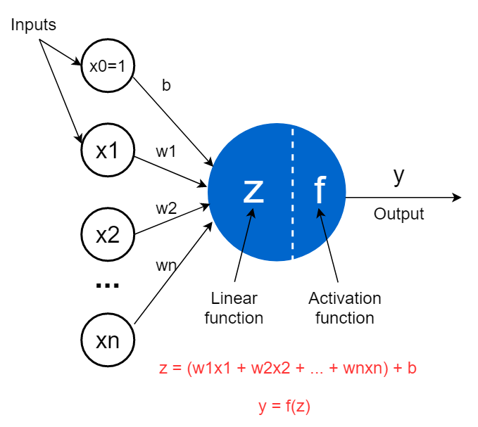
Thus we have

Z = W1*X1 + W2*X2 + W3*X3 ....  Wn*Xn + b ................ eq. 1
Y = f(Z)                           ....................... eq. 2

Here W1, W2…Wn are the weights, b is a bias term which can be assimilated as X0 to the equation with W0 = 1. The bias term ensures that there is discrete value for the weighted sum even if all the inputs are zero. The purpose of the activation function is to introduce non-linearity to the output of the perceptron as otherwise we could only have linear modelling and in real world most real-world data is non-linear. Some popular activation functions include sigmoid, ReLU, and tanh.

To further illustrate the significance of activation function, let us consider a perceptron that has weights [3, -2] and bias = 1. Thus without the activation function the output value Z = 1 + 3X1 - 2X2 where X1 and X2 are the input values. This divides the 2D space into two regions when Z < 0 or Z > 0 essentially a binary classification around the line. This effectively performs binary classification by dividing the input space into two regions. However, without non-linearity, the model cannot capture more complex decision boundaries.

Let’s rewrite the equation using linear algebra as

Y = f(W₀ + XᵀW)

Multi Output perceptron

A single perceptron has limited use, so we construct a network of perceptrons that can take a set of inputs and provide multiple outputs. This works on similar principles as the single perceptron, except in here we define a set of weights that are used for generating one output and similarly another set of weights for next output. The diagram below illustrates a two-output scenario. Note that there can be multiple layers between the input and output layers, commonly referred to as hidden layers.

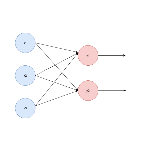
Thus, after dropping the bias term, we have

Yᵢ = f(XᵀWᵢ)  ....................... eq. 3

Where Wᵢ is the weights corresponding to output Yᵢ. The following program shows an implementation of multi layer perceptron using PyTorch. The code is explained through the comments.

import torch
import torch.nn as nn

'''
torch.nn module is the cornerstone of PyTorch for building and
training of neural networks. It abstracts intricate details of
neural network operations enabling a focus on high level design.

torch.nn.Module is the base class for all the neural network
modules. It provides

1. Initialization : Using __init__ to define the layers and
   components of the network.
2. Forward Pass : Using forward to specify how data flows
   through the layers.
3. Parameter Management : Automatically tracks and optimizes
   model Parameters.

The following class defines a simple neural network with one
input, one hidden and a output layer. Essentially it is doing
the following (a code without using torch.nn)

    w1 = torch.randn(input_dim, hidden_dim)
    b1 = torch.randn(1, hidden_dim)

    w2 = torch.randn(hidden_dim, output_dim)
    b2 = torch.randn(1, output_dim)

    def forward(x):
        hidden = torch.matmul(x, w1) + b1
        hidden = torch.relu(hidden)

        output = torch.matmul(hidden, w2) + b2
        return output
'''
class SimpleNN(nn.Module):
    def __init__ (self, input_dim, hidden_dim, output_dim):
        super(SimpleNN, self).__init__()

        # nn.Linear create a fully connected layer that
        # can apply the transformation of Y = X * W + B
        self.hidden = nn.Linear(input_dim, hidden_dim)
        self.output = nn.Linear(hidden_dim, output_dim)

    # This is called from the __call__ method
    def forward(self, input):
        # Apply hidden layer with relu activation function
        x = torch.relu(self.hidden(input))
        # Apply output layer from hidden layer input.
        return self.output(x)


model = SimpleNN(2, 4, 1)

#Example input
x = torch.tensor([1.0, 2.0])
y = model(x)
print("Output with torch.nn is ", y)