A peek into Artificial intelligence - Loss, Gradients and Back propagation
Second installment in AI/ML blogs
In the previous entry, A peek into Artificial intelligence - Part 1, we explored perceptrons, multi-output perceptrons, and their evolution, along with their underlying mathematical foundations. In this post, we’ll take the next step by examining how these foundational concepts can be extended to Deep Neural Networks (DNNs)—mathematical models capable of learning complex patterns from data.
As we have learnt that multi output perceptrons model is a function of multiple inputs and produce multiple outputs. Towards the end we realized that we could have multiple layers in between the input and output layer. Such a model can help with predicting the output given a right set of weights and biases. However the question remains - how to get an accurate set of weights and biases. This is done through the process of training.
Training a neural network involves several steps repeated over time to help the model learn from data. The process starts with a feed-forward pass, where input data moves through the network layer by layer, producing a prediction. This prediction is compared to the true label using a loss function, which quantifies how wrong the prediction is. Then, during backpropagation, the network calculates how each weight and bias contributed to the error. These gradients are used to update the parameters using gradient descent, with the size of each adjustment controlled by the learning rate.
To handle large datasets efficiently, training data is often split into mini-batches—small groups of samples (e.g., 32 or 64 inputs). A batch is just this small chunk of data. One iteration refers to processing a single mini-batch through the full cycle: feed-forward, loss computation, backpropagation, and weight update. Once the model has gone through all mini-batches in the dataset, that completes one epoch. For example, if you have 10,000 training samples and use mini-batches of size 100, each epoch will have 100 iterations. This batching approach allows the model to train efficiently using parallel computation while also smoothing out noise in the gradients, improving convergence and generalization.
The remainder of this article presents the mathematical foundations behind the key steps of neural network training—namely, feed-forward computation, loss calculation, and backpropagation. To make these concepts concrete, we walk through a detailed example that illustrates how these operations are carried out during a single training iteration using a batch size of 1. This step-by-step example demonstrates how data flows through the network, how the error is computed and propagated backward, and how the weights and biases are updated based on the gradients.
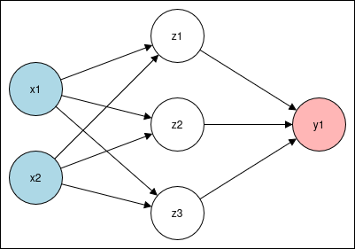
We’ll start by building a simple neural network architecture to demonstrate how feed-forward computation works, step by step.
- Input layer: 2 neurons → x1, x2
- Hidden layer: 3 neurons → z1, z2, z3, using the ReLU activation
- Output layer: 1 neuron → y1, using the Sigmoid activation
Forward pass
To begin, we initialize our input vector and the first layer’s weights and biases as follows:
\[\vec{x} = \begin{bmatrix} x_1 \\ x_2 \end{bmatrix} = \begin{bmatrix} 0.6 \\ 0.4 \end{bmatrix} , \quad W^{(1)} = \begin{bmatrix} 0.2 & -0.3 \\ 0.4 & 0.1 \\ -0.5 & 0.6 \end{bmatrix}, \quad \vec{b}^{(1)} = \begin{bmatrix} 0.1 \\ -0.2 \\ 0.05 \end{bmatrix}\]We compute the pre-activation values in the hidden layer by applying the affine transformation and applying the ReLU activation function, we obtain the hidden layer outputs
\[{a^{(1)}} = W^{(1)} \cdot \vec{x} + \vec{b}^{(1)} = \begin{bmatrix} 0.1 \\ 0.08 \\ -0.01 \end{bmatrix} , \quad \therefore \quad \vec{z^{(1)}} = \text{ReLU}(a^{(1)}) = \begin{bmatrix} \max(0, 0.1) \\ \max(0, 0.08) \\ \max(0, -0.01) \end{bmatrix} = \begin{bmatrix} 0.1 \\ 0.08 \\ 0 \end{bmatrix}\]Next, we calculate the output neuron’s value using a new set of weights and bias for the second (output) layer:
\[\vec{w}^{(2)} = \begin{bmatrix} 0.3 \\ -0.2 \\ 0.5 \end{bmatrix}, \quad b^{(2)} = 0.05\]Using these, we compute the output layer’s pre-activation value and apply the sigmoid function:
\[a^{(2)} = \vec{w}^{(2)} \cdot \vec{z} + b^{(2)} = 0.064 , \quad \therefore \quad \hat{y} = \sigma(a^{(2)}) = \frac{1}{1 + e^{-0.064}} \approx 0.516\]It’s satisfying to see how a neural network processes inputs to generate an output. In our case, the final prediction is $\hat{y}≈0.516$, produced by propagating the input through all the layers using the current set of weights and biases. However, this output may not be accurate—after all, we started with arbitrary weights. Let’s say the true value for the target output y is 1. This difference between the predicted value and the actual value indicates the error the network made.
This marks the end of the feed-forward phase. Next, we move on to compute the loss, which quantifies how far off our prediction is. Broadly, there are two common types of loss functions depending on the task:
- Classification (e.g., predicting 0 or 1):
- Use Binary Cross-Entropy (BCE)
- Regression (e.g., predicting a continuous value):
- Use Mean Squared Error (MSE)
Backward pass
Once we compute the loss, the next step is to adjust the weights in a way that reduces this loss during future predictions. To do this, we need to calculate how sensitive the loss is to each weight—this is where the gradient comes in. Specifically, we compute the gradient of the loss with respect to the weights, starting from the output layer:
\[\frac{\partial \mathcal{L}}{\partial \vec{w}^{(2)}}\]We’re using the binary cross-entropy loss, defined as:
\[\mathcal{L} = - \left( y \cdot \log(\hat{y}) + (1 - y) \cdot \log(1 - \hat{y}) \right)\]Applying the chain rule to compute the derivative with respect to $\vec{w}^{(2)}$
\[\frac{\partial \mathcal{L}}{\partial \vec{w}^{(2)}} = \frac{\partial \mathcal{L}}{\partial \hat{y}} \cdot \frac{\partial \hat{y}}{\partial a^{(2)}} \cdot \frac{\partial a^{(2)}}{\partial \vec{w}^{(2)}}\]We evaluate each term individually:
\[\frac{\partial \mathcal{L}}{\partial \hat{y}} = - \left( \frac{y}{\hat{y}} - \frac{1 - y}{1 - \hat{y}} \right)\] \[\frac{\partial \hat{y}}{\partial a^{(2)}} = \hat{y}(1 - \hat{y}) \quad as \quad \hat{y} = \sigma(a^{(2)})\] \[and \quad \frac{\partial a^{(2)}}{\partial \vec{w}^{(2)}} = \vec{z}^{(1)} \quad as \quad \ a^{(2)} = \vec{w}^{(2)} \cdot \vec{z}^{(1)} + b^{(2)}\] \[\therefore \frac{\partial \mathcal{L}}{\partial \vec{w}^{(2)}} = - \left( \frac{y}{\hat{y}} - \frac{1 - y}{1 - \hat{y}} \right) \cdot \hat{y}(1 - \hat{y}) \cdot \vec{z}^{(1)}\]Simplifying
\[- \left( \frac{y}{\hat{y}} - \frac{1 - y}{1 - \hat{y}} \right) \cdot \hat{y}(1 - \hat{y}) = \hat{y} - y \implies \frac{\partial \mathcal{L}}{\partial \vec{w}^{(2)}} = (\hat{y} - y) \cdot \vec{z}^{(1)}\]if we substitute $\delta^{(2)} = \hat{y} - y$ then we have
\[\boxed { \frac{\partial \mathcal{L}}{\partial \vec{w}^{(2)}} = \delta^{(2)} \cdot \vec{z}^{(1)} } \quad \quad --- eq. 1\]Now let’s compute the gradient with respect to the bias in the output layer. Again, we use the chain rule:
\[\frac{\partial \mathcal{L}}{\partial {b}^{(2)}} = \frac{\partial \mathcal{L}}{\partial \hat{y}} \cdot \frac{\partial \hat{y}}{\partial a^{(2)}} \cdot \frac{\partial a^{(2)}}{\partial \vec{b}^{(2)}}\] \[\quad \frac{\partial a^{(2)}}{\partial {b}^{(2)}} = 1 \quad as \quad \ a^{(2)} = \vec{w}^{(2)} \cdot \vec{z}^{(1)} + b^{(2)}\] \[\boxed { \frac{\partial \mathcal{L}}{\partial b^{(2)}} = \hat{y} - y \quad \implies \delta^{(2)} } \quad \quad --- eq. 2\]Backpropagate to hidden layer
Now that we’ve computed the gradients for the output layer, the next step is to backpropagate the loss to the hidden layer so we can update the input weights $\vec{w}^{(1)}$. To compute the gradient of the loss with respect to the input layer weights, we again apply the chain rule:
\[\frac{\partial \mathcal{L}}{\partial \vec{w}^{(1)}} = \frac{\partial \mathcal{L}}{\partial \vec{z}^{(1)}} \cdot \frac{\partial \vec{z}^{(1)}}{\partial \vec{a}^{(1)}} \cdot \frac{\partial \vec{a}^{(1)}}{\partial \vec{w}^{(1)}}\]Let’s compute each component step by step. First, we compute the gradient of the loss with respect to the hidden layer output $\vec{z}^{(1)}$. This comes from the gradient at the output layer:
\[\frac{\partial \mathcal{L}}{\partial \vec{z}^{(1)}} = \frac{\partial \mathcal{L}}{\partial a^{(2)}} \cdot \frac{\partial a^{(2)}}{\partial \vec{z}^{(1)}}\]As $\hat{y} = \sigma(a^{(2)})$ and $\mathcal{L} = -\left[y \log(\hat{y}) + (1 - y)\log(1 - \hat{y})\right]$, we have
\[\frac{\partial \mathcal{L}}{\partial a^{(2)}} = \hat{y} - y = \delta^{(2)}\]and since $a^{(2)} = \vec{w}^{(2)} \cdot \vec{z}^{(1)} + b^{(2)}$ and $\frac{\partial a^{(2)}}{\partial \vec{z}^{(1)}} = \vec{w}^{(2)}$, we have
\[\begin{aligned} \frac{\partial \mathcal{L}}{\partial \vec{z}^{(1)}} = \frac{\partial \mathcal{L}}{\partial a^{(2)}} \cdot \frac{\partial a^{(2)}}{\partial \vec{z}^{(1)}} = \delta^{(2)} \cdot \vec{w}^{(2)} \end{aligned}\]Next, we compute the derivative of the ReLU activation. Since $\vec{z}^{(1)} = \text{ReLU}(\vec{a}^{(1)})$, we have
\[\frac{\partial \vec{z}^{(1)}}{\partial \vec{a}^{(1)}} = \text{ReLU}'(\vec{a}^{(1)}) = \begin{cases} 1 & \text{if } a_i^{(1)} > 0 \\ 0 & \text{otherwise} \end{cases}\]We now define the hidden layer error signal as:
\[\delta^{(1)} = \frac{\partial \mathcal{L}}{\partial \vec{a}^{(1)}} \implies \frac{\partial \mathcal{L}}{\partial \vec{z}^{(1)}} \cdot \frac{\partial \vec{z}^{(1)}}{\partial \vec{a}^{(1)}} \implies \delta^{(1)} = \left( \vec{w}^{(2)} \cdot \delta^{(2)} \right) \odot \text{ReLU}'\left( \vec{a}^{(1)} \right)\] \[\boxed {\frac{\partial \mathcal{L}}{\partial \vec{w}^{(1)}} = \delta^{(1)} \otimes \vec{x}^T } \quad as \quad a^{(1)} = \vec{w}^{(1)} \cdot \vec{x} + b^{(1)} \quad \quad --- eq. 3\]We’ll follow a similar approach to compute the gradient with respect to the bias term next.
\[\boxed {\frac{\partial \mathcal{L}}{\partial \vec{b}^{(1)}} = \delta^{(1)} } \quad \quad --- eq. 4\]Now that we’ve derived the gradient expressions in equations (1) through (4), we can proceed to apply backpropagation to our network using the values computed above. Previously, we calculated the binary cross-entropy loss as: $\mathcal{L}_{\text{BCE}} = -\left[ y \cdot \log(\hat{y}) + (1 - y) \cdot \log(1 - \hat{y}) \right] = -\log(0.516) \approx 0.661$.
We also know from earlier that the error signal at the output layer is: $\delta^{(2)} = \hat{y} - y$, thus we have $\delta^{(2)} = -0.4840$.
We will compute the gradients with respect to output weights and bias from equation 1 and 2.
\[\frac{\partial \mathcal{L}}{\partial \vec{w}^{(2)}} = \delta^{(2)} \cdot \vec{z}^{(1)} = \begin{bmatrix} -0.0484 \\ -0.0387 \\ 0 \end{bmatrix} , \quad \frac{\partial \mathcal{L}}{\partial b^{(2)}} = -0.4840\]To back-propagate into the hidden layer, we compute the hidden layer error signal:
\[\delta^{(1)} = \left( \vec{w}^{(2)} \cdot \delta^{(2)} \right) \odot \text{ReLU}'(\vec{a}^{(1)})\]We already know:
\[\vec{w}^{(2)} \cdot \delta^{(2)} = -0.48401 \cdot \begin{bmatrix} 0.3 \\ -0.2 \\ 0.5 \end{bmatrix} = \begin{bmatrix} -0.1452 \\ 0.0968 \\ -0.2420 \end{bmatrix}, \quad \text{ReLU}'(\vec{a}^{(1)}) = \begin{bmatrix} 1 \\ 1 \\ 0 \end{bmatrix}\] \[\therefore \quad \delta^{(1)} = \begin{bmatrix} -0.1452 \\ 0.0968 \\ 0 \end{bmatrix}\]Now, using this $\delta^{(1)}$, we calculate the gradient of the loss with respect to the input weights $\vec{w}^{(2)}$:
\[\frac{\partial \mathcal{L}}{\partial W^{(1)}} = \delta^{(1)} \cdot \vec{x}^T = \begin{bmatrix} -0.1452 \\ 0.0968 \\ 0 \end{bmatrix} \cdot \begin{bmatrix} 0.6 & 0.4 \end{bmatrix} = \begin{bmatrix} -0.08712 & -0.05808 \\ 0.05808 & 0.03872 \\ 0 & 0 \end{bmatrix}\]Similarly for bias we have
\[\frac{\partial \mathcal{L}}{\partial \vec{b}^{(1)}} = \begin{bmatrix} -0.1452 \\ 0.0968 \\ 0 \end{bmatrix}\]Weight Update Rule
Finally, to update the weights and biases using gradient descent, we apply the following update rule for each parameter $\theta \in { W^{(1)}, b^{(1)}, W^{(2)}, b^{(2)} }$, the update rule is:
\[\theta := \theta - \eta \cdot \frac{\partial \mathcal{L}}{\partial \theta}\]where $\eta$ is the learning rate.
\[\vec{w}^{(2)}_{\text{new}} = \begin{bmatrix} 0.3 \\ -0.2 \\ 0.5 \end{bmatrix} - 0.1 \cdot \begin{bmatrix} -0.0484 \\ -0.0387 \\ 0 \end{bmatrix} = \begin{bmatrix} 0.30484 \\ -0.19613 \\ 0.5 \end{bmatrix}\] \[\vec{w}^{(1)}_{\text{new}} = \begin{bmatrix} 0.2 & -0.3 \\ 0.4 & 0.1 \\ -0.5 & 0.6 \end{bmatrix} - 0.1 \cdot \begin{bmatrix} -0.08712 & -0.05808 \\ 0.05808 & 0.03872 \\ 0 & 0 \end{bmatrix} = \begin{bmatrix} 0.208712 & -0.294192 \\ 0.394192 & 0.096128 \\ -0.5 & 0.6 \end{bmatrix}\] \[b^{(2)}_{\text{new}} = 0.05 - 0.1 \cdot (-0.4840) = 0.0984\] \[\vec{b}^{(1)}_{\text{new}} = \begin{bmatrix} 0.1 \\ -0.2 \\ 0.05 \end{bmatrix} - 0.1 \cdot \begin{bmatrix} -0.1452 \\ 0.0968 \\ 0 \end{bmatrix} = \begin{bmatrix} 0.11452 \\ -0.20968 \\ 0.05 \end{bmatrix}\]After calculating the gradients and updating the weights and biases using the gradient descent rule, the neural network is ready for the next iteration of training. This means the updated parameters are used to perform a new forward pass with either the next input sample or batch of samples. The network predicts outputs based on these updated weights, calculates the loss again, and back-propagates the error to further refine the weights. This iterative cycle continues — feeding forward, calculating loss, back-propagating, and updating parameters — until the network’s performance improves sufficiently, typically measured by the loss decreasing to a satisfactory level or after a fixed number of training epochs.